Visualizing linear systems of ODEs
Last edited at 2025-06-07
72 Views
(공학수학1 과제용)
Let's visualize some linear systems of ODEs with Python.
We will draw the phase portraits of ODEs and the solution curves from given inital conditions.
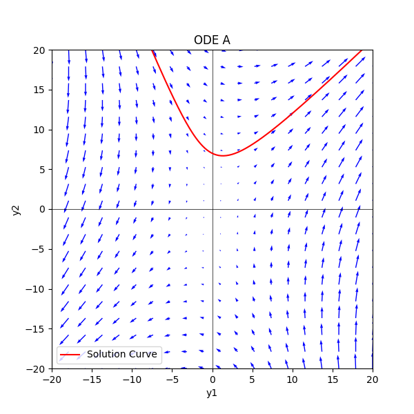
ODE (a)
Initial conditions:
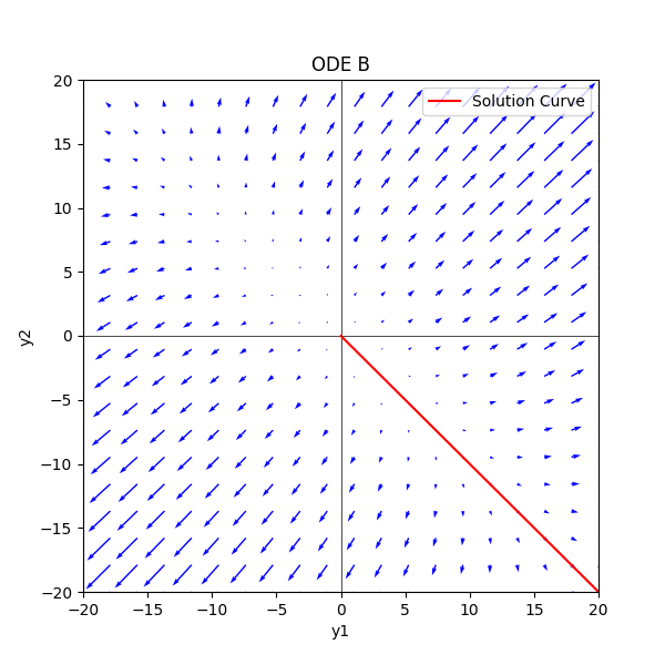
ODE (b)
Initial conditions:
Source Code (Python)
import matplotlib.pyplot as plt
import numpy as np

def draw_ode(title, ode, sol, plotRange=(-20, 20)):
    plt.figure(figsize=(6, 6))
    plt.title(title)

    plt.xlim(plotRange)
    plt.ylim(plotRange)
    plt.xlabel('y1')
    plt.ylabel('y2')

    plt.axhline(0, color='black', lw=0.5)
    plt.axvline(0, color='black', lw=0.5)

    draw_phase_portrait(ode, plotRange)
    draw_sol(sol)

    plt.show()


def draw_phase_portrait(ode, plotRange, num_points=20):
    y1 = np.linspace(plotRange[0], plotRange[1], num_points)
    y2 = np.linspace(plotRange[0], plotRange[1], num_points)
    Y1, Y2 = np.meshgrid(y1, y2)

    Y1 = Y1.flatten()
    Y2 = Y2.flatten()
    Dy1, Dy2 = ode(Y1, Y2)
    Dy1 = np.reshape(Dy1, (num_points, num_points))
    Dy2 = np.reshape(Dy2, (num_points, num_points))

    plt.quiver(Y1, Y2, Dy1, Dy2, color='blue')

def draw_sol(sol):
    t = np.linspace(-5, 5, 1000)
    y1, y2 = sol(t)

    plt.plot(y1, y2, label='Solution Curve', color='red')
    plt.legend()


def ode_a(y1, y2):
    A = np.array([[2, 2], [5, -1]])
    return np.dot(A, np.array([y1, y2]))
def sol_a(t):
    y1 = -2*np.exp(-3*t) + 2*np.exp(4*t)
    y2 = 5*np.exp(-3*t) + 2*np.exp(4*t)
    return np.array([y1, y2])


def ode_b(y1, y2):
    A = np.array([[3, 2], [2, 3]])
    return np.dot(A, np.array([y1, y2]))
def sol_b(t):
    y1 = 1*np.exp(t)
    y2 = -1*np.exp(t)
    return np.array([y1, y2])


if __name__ == "__main__":
    draw_ode('ODE A', ode_a, sol_a)
    draw_ode('ODE B', ode_b, sol_b)